Next Year Already?

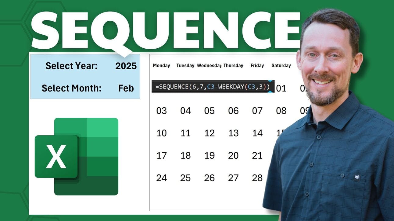
In today’s lesson:

1. Sequence Function

2. + Dropdown Menu

3. = Dynamic Calendar

MAIN ARTICLE

Video walkthrough:

What is Sequence?

Sequence is a quick way to create a sequence of numbers…or in our case, dates.

It takes at least one argument, and up to four:

Sequence(rows, [columns], [start], [step])

It at least needs to know how many rows of data you want. If that’s all you give it, it’ll simply return a sequence of numbers from 1 to whatever number you enter. SEQUENCE(4) returns the numbers 1, 2, 3, 4 in four rows.

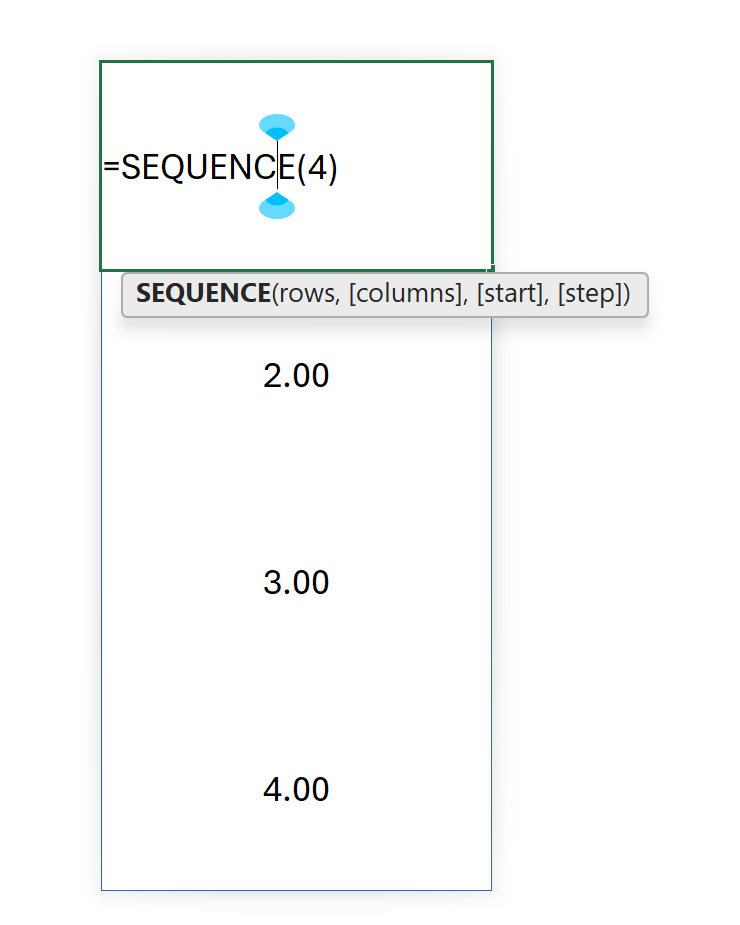
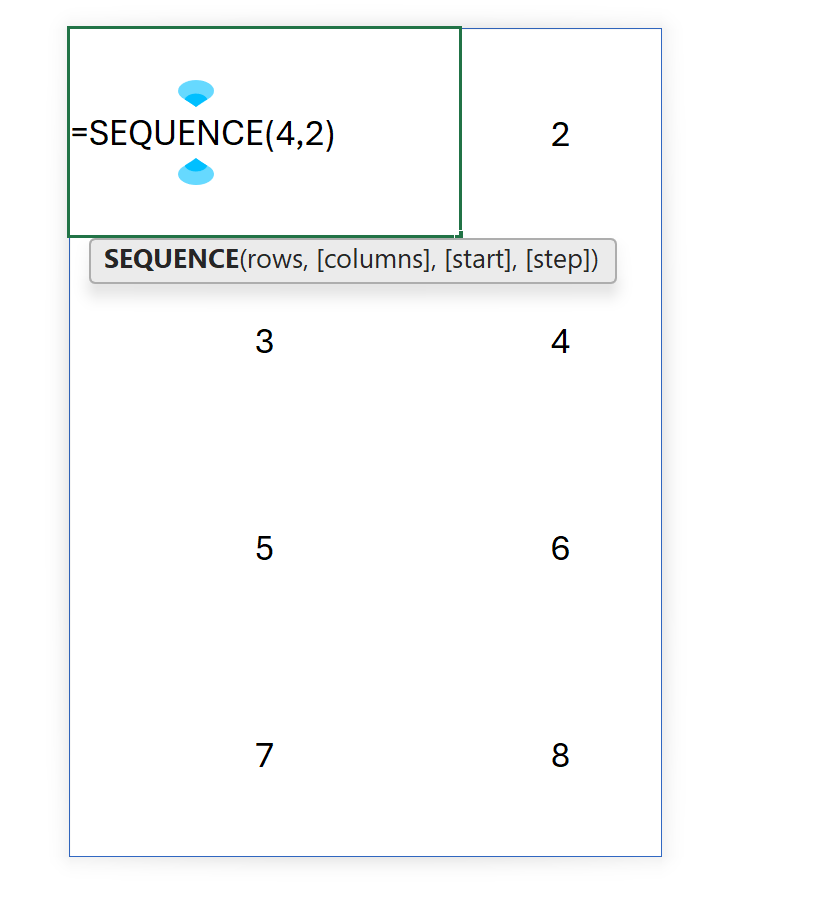
Add an argument for columns and it’ll continue the sequence through to however many columns you specify:

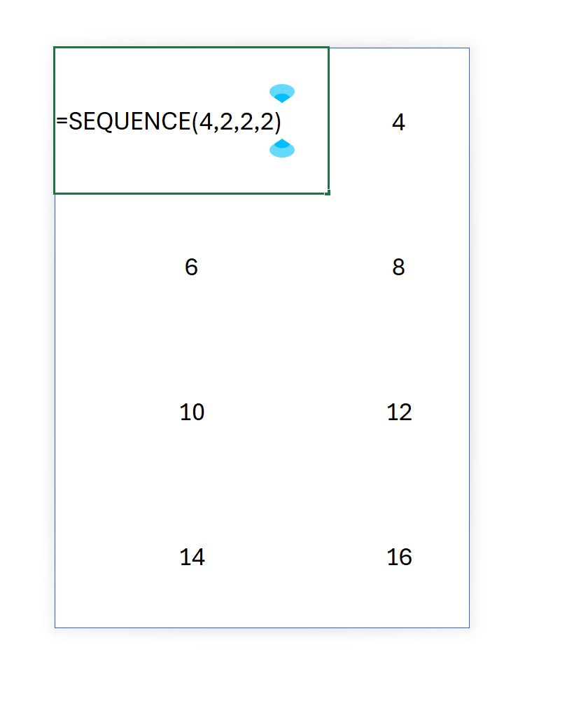
Finally, adding a start and step argument will tell the sequence where to start (if you want it to be other than the number 1) and what you want to increment by:

Let’s make one more sequence that we’ll use in the following step.

I want to be able to type any year, and then write a sequence that will return the first days of the month of that year.

We could type it all out, but a simple sequence makes it easy. And from now on, we only have to change the year:

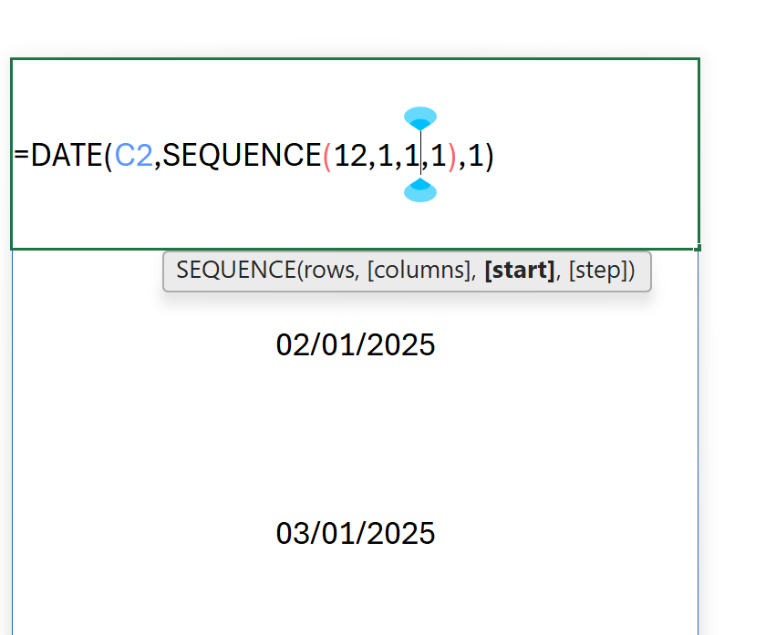
=DATE(C1,SEQUENCE(12,1,1,1),1)

This pulls the date from C2 as the year and then uses Sequence inside the Date function to go through each of the 12 months one at a time and return only the first day of each month.

Date Dropdown Selection

We want to use Sequence to make a dynamic calendar. Let’s create a dropdown list of the first days of each month of the year.

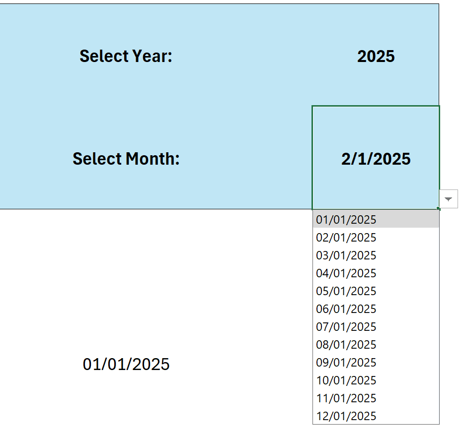
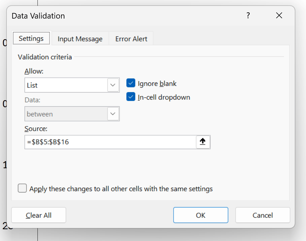
In cell C3, we’ll select Data - Data Validation - Data Validation.

We’ll select Allow from a List.

Then we’ll have our Source be a list of the first days of the months of the year. I wrote mine in cells B5:B16 in the example below.

Sequence for a Month Calendar

Now we can select a year and a month. Let’s populate an actual calendar with that month’s data.

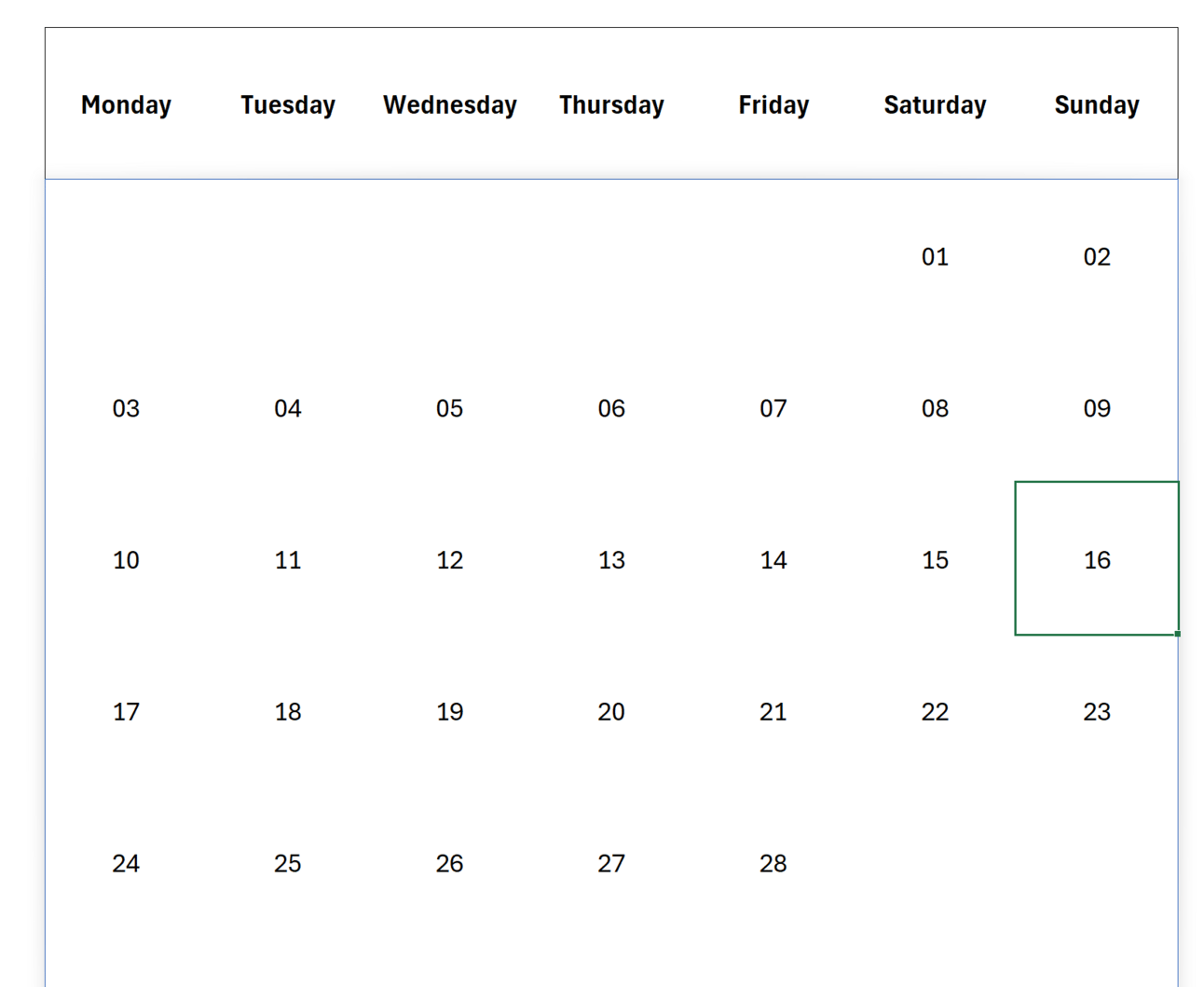
The sequencing is tricky because we want the dates to line up with the days of the week.

The first arguments for rows and columns are 6 and 7.

Six rows because there can be instances where the first of the month is on a Saturday or Sunday and the end of the month could then fall onto the 6th week.

Seven columns because seven days in a week. Duh.

=SEQUENCE(6,7,C3-WEEKDAY(C3,3))

Now it gets tricky, though. We don’t just want to start with 1 because the first of the month won’t always be on a Monday. Instead, we need to manipulate the start value so that it lines up with that Monday.

Take February 2025. The first of the month is Saturday, so we want to count backwards 5 days to January 27th for that first slot in our calendar. (We’ll clean it up later with conditional formatting, so it looks blank).

So, we use some math magic.

The Weekday function can return in numerical format which weekday is represented by a date. WEEKDAY(C3,3) returns 5 since Saturday is the 5th day in the week in this sequence. The argument 3 specifies the return type where Monday is 0 and Saturday is 5.

All we have to do now is take C3 and subtract the five days we found in the Weekday formula.

This is dynamic since it will work no matter which year and month we select.

Conditional Formatting

Only thing missing is some formatting. Let’s make it look like the calendar squares are blank for all the dates before and after the current month.

We only need two custom formulas for this to work. One for the first line of our calendar where the first day of the month will vary, and one for the last two lines where the last day of the month will fall.

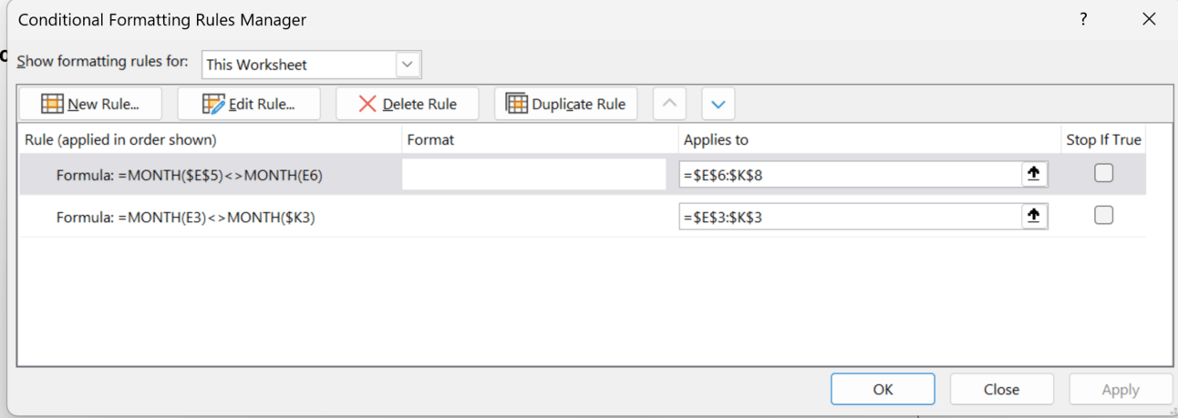
First, let’s open the conditional formatting window by selecting Home - Conditional Formatting - New Rule.

For our top line, we need to check that the month of each day against the month of the current calendar view.

=MONTH(E3)<>MONTH($K3)

To do this, we take a day that will definitely be in the current month (K3 since that’s the last day of the week on that first line) and compare whether that’s equal to the month of the rest of the days in that line.

We use the month function and the <> comparison to check. We lock $K3 in place with the dollar sign but leave E3 alone so that it’ll check each column of the row.

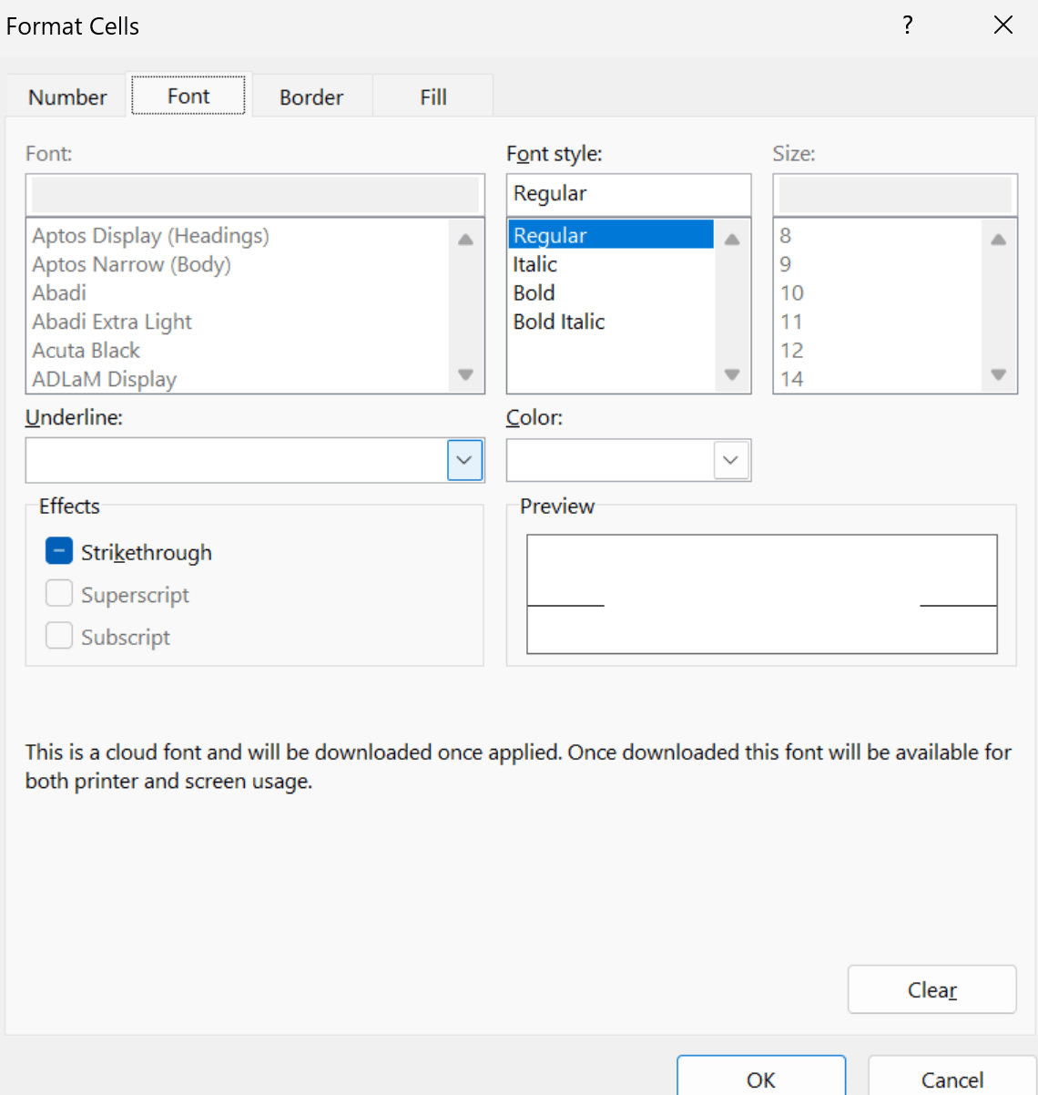
Then we set the formatting to whatever we want. In my case, I put it as white text so it just disappears on the white background.

We apply this to the range $E$3:$K$3 and we’re good to go.

We then do the same thing to the last two rows of our calendar by applying the same rule to the range $E$6:$K$8.

Here’s the video link again in case you’re scratching your head on any of the steps. There are chapter markers on the video so you can easily skip to whatever part you need help with.

Learn without limits on Coursera.
Google’s latest course is Prompting Essentials. Learn to give clear and specific instructions to generative AI in 5 easy steps.
Enroll here.

NEXT STEPS

Whenever you’re ready, here’s how I can help:

1. Business tech stack (FREE)
   My recommendations for software and tools I use to create content and run my online business.

2. Sponsor Got Sheet
   Got Sheet teaches business operators, teachers and entrepreneurs how to get good at spreadsheets. Interested in sponsoring an issue or a series of Got Sheet newsletters? Reach out to get more information.

3. Personal budget tool
   As a Got Sheet subscriber, I want you to have a 75% discount on the personal budget I built 10+ years ago and am still using to this day.

HAPPY SPREADSHEETING!

Enjoyed this issue?
Subscribe below or Leave a testimonial

Cheers, Eamonn
Connect on LinkedIn, YouTube & Twitter.