Importing Data to Google Sheets (post 1 of 3)

This is post 1/3 in the Import Series.

Google Sheets has five built-in functions to import data from various sources into your sheet.

1. IMPORTRANGE(spreadsheet_url, range_string)

2. IMPORTHTML(url, query, index)

3. IMPORTDATA()

4. IMPORTFEED()

5. IMPORTXML()

Each of these pulls data from other sources. This could be another spreadsheet, an RSS feed, or a website. We’ll look at two of them today: IMPORTRANGE() and IMPORTHTML().

Video Walkthrough

IMPORTHTML

This takes the URL for a website and then returns either a “list” or a “table”.

This function requires the data to be in a certain format (list or table), and we’ll have to use another function if our data isn’t in one of those formats.

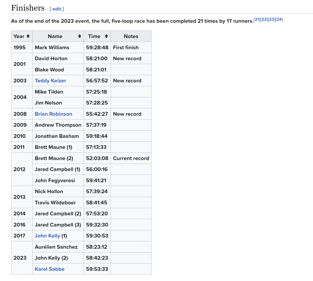
Let’s look at a list of the finishers of the Barkley Marathons😀 

This is a table over on Wikipedia, and by using the url in our spreadsheet, we can bring each cell’s data into our spreadsheet.

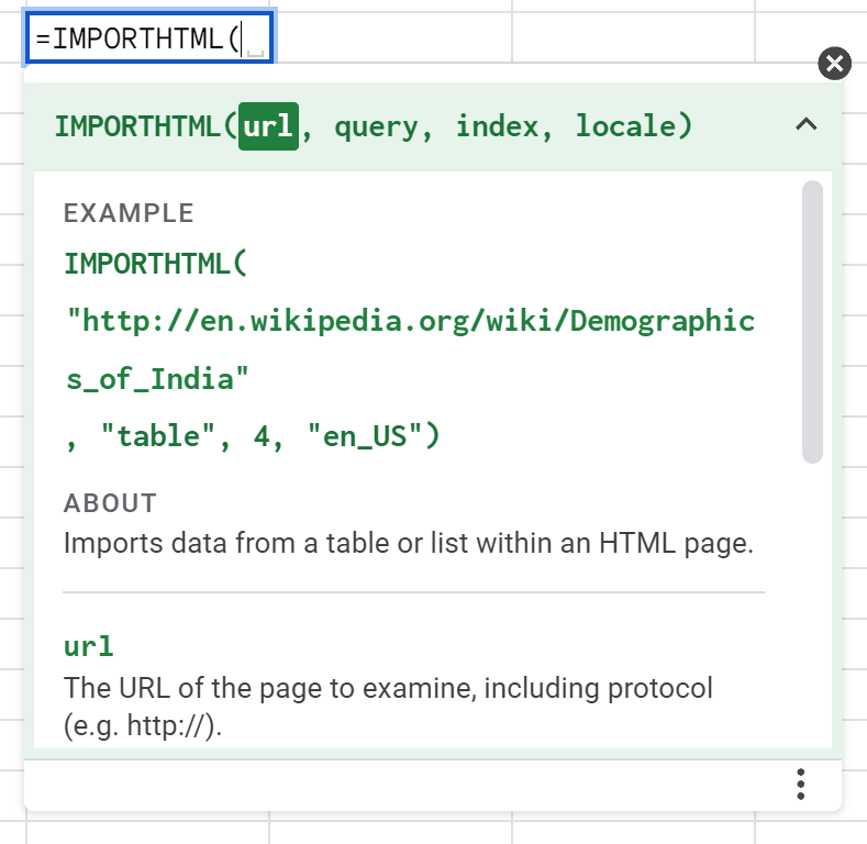
The url and the query are straightforward. We need the url of the page and the type of query (this will either be “table” or “list” and it does have to be in quotes.

The index is simply the index of the table or list on the page. If there are multiple tables on the page, then you need to specify which one to pull over, otherwise it will just grab the first one.

Be aware that the index begins with index 0 rather than 1.

I’ve opted to put the url in a cell so that the actual function is a little more readable as I reference the URL in cell B3:

=IMPORTHTML(B3,"table",0)

If the data you’re looking for is in a list rather than a table, you would use the same technique to get it and simply have “list” as the second argument in the function.

IMPORTRANGE(spreadsheet_url, range_string)

If you’ve ever wondered whether you can connect two Google Sheets to one another, this is the function for you!

I’ve used it extensively in an inventory management scenario where several sheets need to order from a master sheet.

The IMPORTRANGE function allows us to give it a url of the spreadsheet and a range that we want to grab.

We can either type the url in manually and enclose it in quotes:

=IMPORTRANGE("https://docs.google.com/spreadsheets/d/1S0H1FDHBC_7oxe2NCpnfuJcklaLpYCFuo_eRhADnyWg/edit#gid=0","sheet1!a1:K")

Or, as we did with the Barkley example, we can put the url in a cell and then reference it for a cleaner formula:

=IMPORTRANGE(B2,"data!a1:K")

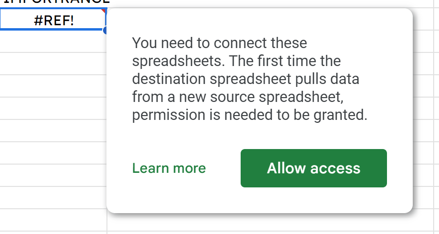
The first time that we use this to connect two spreadsheets, we will be prompted to allow access:

Once we do, though, all of our data will be brought over.

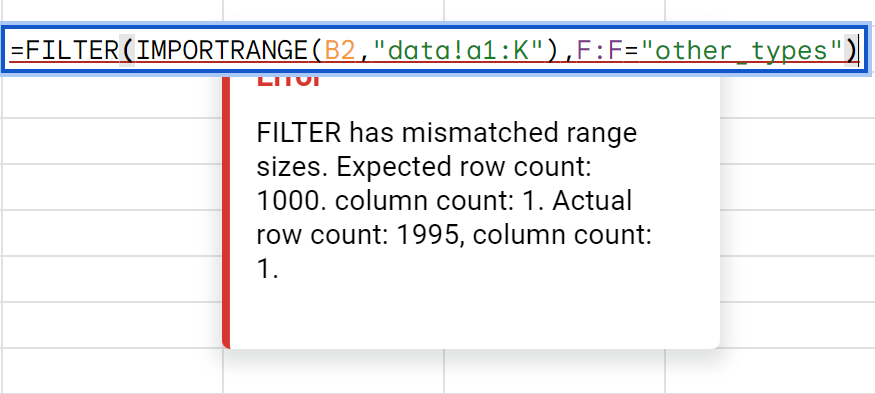
We can even filter the data as we bring it over, although we’ll have to make sure to match up the row numbers of the imported data with the row count in our current spreadsheet:

To get around this, we simply need to ensure that we’re using matched range sizes for our filter.

=FILTER(IMPORTRANGE(B2,"data!a1:K"),F4:F1003="other_types")

More IMPORTS

Next time, we’ll go through IMPORTDATA() and IMPORTFEED().

Happy sheeting until then!